


Data Processing
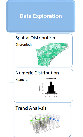
During the data exploration segment of the research, a variety of methods were used to better visualize and understand the data for further statistical analysis. In order to understand the spatial distribution of the variables, choropleth maps were used. Histograms were used to model numeric distribution curves. Finally, trend analysis was performed on the data in order to further detect spatial patterns. Ultimately, the exploration helped to determine areas within the data to focus on during the later analysis phase to determine statistical significance.
Data Exploration and Analysis
All of the data was collected from a variety of sources, in order to analyze the three main chronic conditions identified for North Carolina, South Carolina, and Georgia.
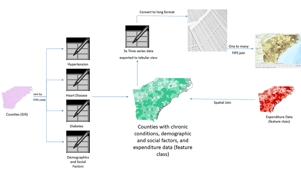
The initial counties layer, which included the county boundaries and basic demographic information for each county, was collected as a shapefile from ESRI. The data was collected based on the five-digit Federal Information Processing Standard (FIPS) code. The FIPS code uniquely identifies counties in the United States. The FIPS code enable data to be joined from multiple sources to create a large data set with data linked to each county based on the unique FIPS code.
The tabular data was joined by FIPS code to the original GIS layer shapefile to create a master data table and include the geometry of each county. The tabular data includes heart disease, hypertension, diabetes, and some demographic data. Demographic data includes household income, medical insurance coverage, medical visits, fast food expenditures, fruit and vegetable expenditures, and others.
The final source that included expenditure habits did not have an associated FIPS code but already was in a GIS feature layer. To add this source to the master table, that contains the tabular data and the original GIS file, a spatial join was used.
Temporal data was added to the original GIS shapefile with a FIPS code. The data was exported to a new Excel sheet to be edited in OpenRefine. By using OpenRefine, the time series data was extracted to one column and added back to the original GIS shapefile with a one-to-many join. The new file was then animated as a time series.
Weighted Chronic Conditions Index for Heart Disease, Hypertension, and Diabetes
Data analysis was used to determine if there was statistical significance in the areas of interest discovered during the exploration phase. Spatial autocorrelation was used to determine if there was actual statistical clustering within the data using a z-score. Incremental spatial autocorrelation was then used to determine distance interval for further analysis. Once clustering was discovered and the interval was determined, an optimized hot spot analysis was run to determine where the clustering was. Hot spots seek to show high number of high values and cold spots show high numbers of low values grouped in a spatial area. The optimized hot spot analysis gave us a more specific interval to run a more focused hot spot analysis and then an outlier analysis to eliminate extremes from the data. Following the hot spot modeling, a variety of methods were used to determine variables possibly correlated with the hot and cold spots. A scatterplot matrix was created with a variety of variables in order to show trends. Ordinary Least Squares (OLS), exploratory regression, and geographic weighted regression (GWR) analysizes were also used to normalize data to a trend.
An index was created in order to show how much each individual disease contributed to our overall research goal of chronic conditions. Each disease was given an equal weight in showing chronic conditions.
Data Exploration
Data Analysis